Flame Front Dynamics
Hele-Shaw burner
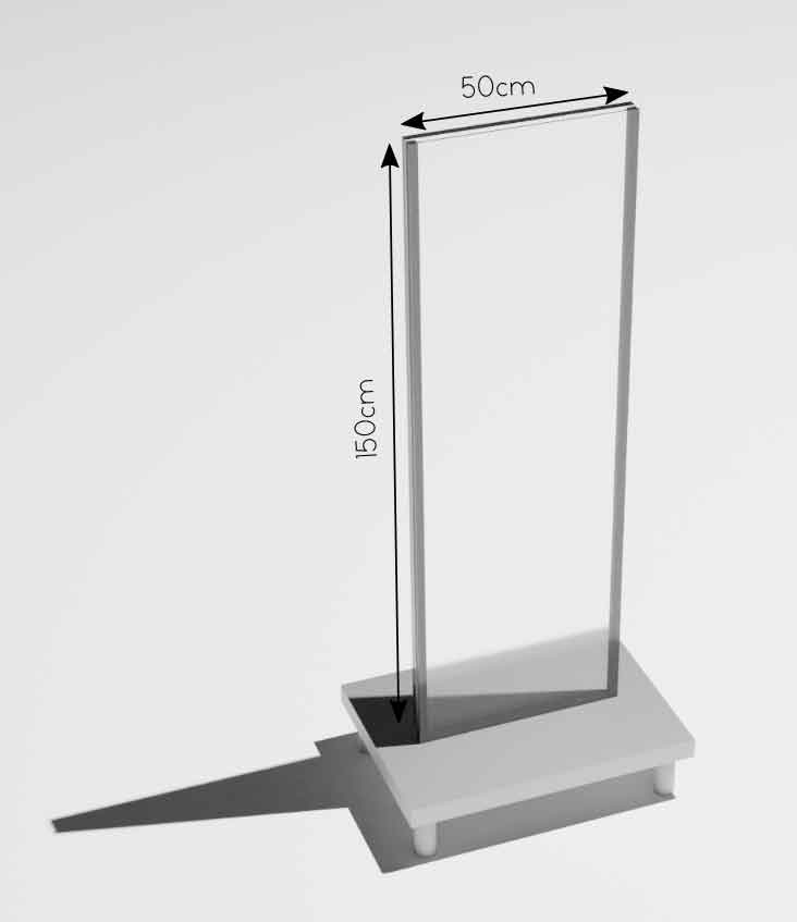
Fig. 1: 3D model of the Hele-Shaw burner employed in this study.
The burner is composed of two borosilicate glass plates that are 1500 mm in height and 500 mm in width. These plates are vertically oriented parallel to each others and separated by a 5 mm gap with the help of two vertical spacers positioned along the vertical sides. The all thing is clamped on a rigid aluminium base and forms a volume that is closed on the sides and at the bottom and opened at the top. This volume can be filled with a reactive mixture (methane-air, propane-air) whose equivalence ratio is controlled with the help of mass flow regulators. Flames are ignited from the top of the burner and propagates downwards until all the reactive mixture has burnt. The flame dynamics is visualized through one of the two glass plates with a high-speed video camera.
Thanks to the confined geometry offered by this apparatus, the shape of the flame front quickly reach a stationnary state in the direction corresponding to the shortest dimension of the burner and the dynamics take place only in the plane of the two larger dimensions, therefore facilitating the visualization.
Vid. 1: When the flame propagates downwards in the burner, it exhibits these typical cellular structures separated by sharp "cusps" pointing towards the burnt gases. The width of the field of view (from the left end to the right end of the front) here is about 50 cm.
Vid. 2: These cellular structures evolve through complex dynamics that involve merging of existing cells and creation of new ones. Their evolution can be visualized by superimposing flame front configurations at different instants in time on the same image. These dynamics result from a competition between different mechanisms.
Darrieus-Landau instability
The main mechanism involved is the one that makes the planar flame configuration unstable. It results from the fact that: (i) the flame propagates with a non-zero speed relatively to the unburnt gases (ii) the flow undergo a density "drop" when passing through the flame.
(i) A premixed flame is a self sustained chemical reaction that propagates through the reactive mixture. A planar flame propagates towards the unburnt gases perpendicular to itself at a speed \(u_1^\perp=u_L\) called laminar flame speed. (ii) Due to the energy released by the chemical reaction, the flow undergoes a sudden temperature "jump" when passing through the flame which results in a density drop between the flow ahead (of density \(\rho_1\)) and the flow behind (of density \(\rho_2\)) the flame.
For the mass to be conserved despite this density contrast \(\gamma=(\rho_1-\rho_2)/\rho_1\), the magnitude of the flow speed has to increase from \(|u_1|\) to \(|u_2|=|u_1|/(1-\gamma)\) when passing through the reactive interface. As momentum conservation and mass conservation impose continuity of the speed in the tangential direction to the interface, the increase in speed must occur along the normal to the interface. For particles of fluid passing through the interface with a non zero incidence angle this results in a deviation of their trajectories (see Fig. 2). This phenomena is similar to the refraction of a beam of light passing through an interface separating two medium with two different refraction indices.
Due to the deviation of the fluid particles at the interface the flow speed increases (respectively decreases) ahead the concave (respectively convex) parts of the flame front (see Fig. 3). If the flame propagates normally to itself with the same speed everywhere, this results in an amplification of any perturbation of the planar flame front.
The deviation of the streamlines and the density drop at the interface can be visualized by seeding the reactive mixture with micrometric solid particles that act as passive tracers of the flow. The flow is then illuminated with a laser sheet. Fig. 4 shows a visualization of the flow passing through a propane-air flame.
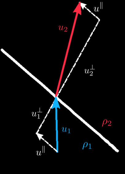
Fig. 2: Deviation of the flow lines at the interface. The increase in speed occurs along the normal to the interface due to conservation of the speed in the tangential direction.
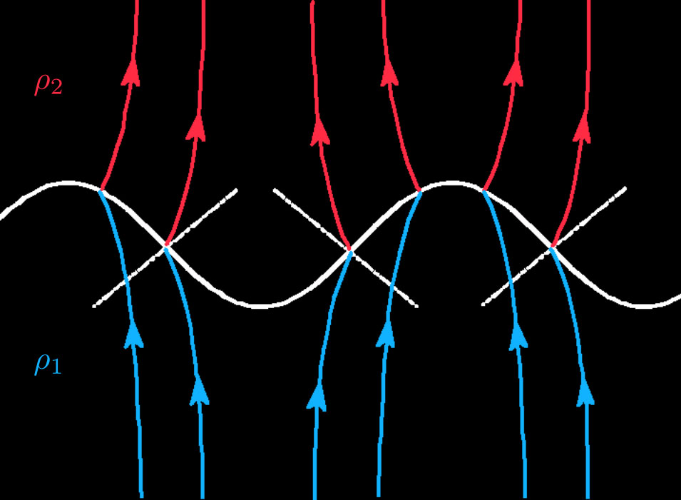
Fig. 3: Schematic of the streamlines passing through a curved interface. The blue (respectively red) lines correspond to the unburnt (respectively burnt) gases streamlines.
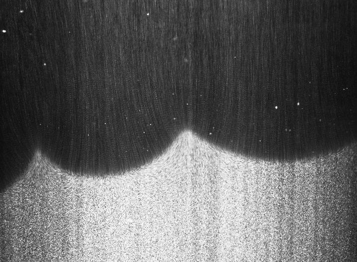
Fig. 4: Propane air-flame propagating downwards in a Hele-Shaw burner. The density jump and the deviation of the streamlines at the interface are readily visible. The width of the field of view is about 5 cm.
This phenomena, known as "Darrieus-Landau instability", was discovered independently by Darrieus and Landau. In their model, they considered the flame as a density interface of infinitesimal thickness separating two inviscid and incrompressible flows with different densities. One of their assumption was to consider that the flame propagates everywhere normally to itself towards the unburnt gases at the laminar speed \(u_L\). Under these assumptions, the problem involves only a speed of propagation \(u_L\) and a density contrast \(\gamma\). A simple dimensional analysis implies that the growth rate of an harmonic perturbation with wavenumber \(k\) must be of the form: $$\sigma=\Omega(\gamma)u_L \left|k\right|,$$ where \(\Omega(\gamma)\) is a function of \(\gamma\) that vanishes for \(\gamma=0\). Its detailed expression is obtained by performing a linear stability analysis of the problem described above (see Clavin & Searby (2016) for example).
Transport phenomena in the thickness of the flame
In practice, the assumption that the flames propagates at the same speed \(u_L\) everywhere is valid only if the wavelength \(\lambda=2\pi/k\) of the perturbation and the smallest scale associated with the background flow are small compared to the thickness of the flame \(d_L\). If one of these length scales becomes \(O(d_L)\), the tranport phenomena happening in the thickness of the flame in the parallel direction to the flame front play an important role on the dynamics of the flame and are likely to modify the standard Darrieus-Landau picture described above.
Heat transport
Heat transport phenomena in the direction parallel to the direction of propagation are likely to affect the local flame speed. This is easily seen by looking at a flat flame submitted to an harmonic perturbation with wavelength \(\lambda=O(d_L)\) (see Fig. 5).
Even in the absence of a background flow, the flame generates its own flow through deviation of the streamlines due to the Darrieus-Landau effect discussed earlier. This induces advective fluxes in the direction parallel to the flame that tend to transport heat from the convex parts of the flame to the concave ones (see Fig. 5). As the reaction rate is a strongly dependent function of the local temperature, the flame tends to consume the reactive products (and propagates faster) in the concave parts than in the convex ones.
In addition, the temperature inhomogeneities generate diffusive fluxes that also tend to remove heat from the convex parts and bring it to the concave ones (see Fig. 5).
Therefore, both the advective heat fluxes due to the flow generated by the flame and the diffusive heat fluxes tend to increase the local flame speed in the part that are behind (concave) and decrease it in the part that are ahead (convex) and have therefore a stabilizing effect. However, we note that in the presence of an inhomogeneous background flow, the latter could overcome the flow induced by the flame itself and have the opposite effect.
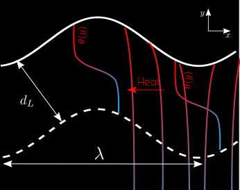
Fig. 5: Heat transport phenomena in the flame. The thickness of the flame is materialized by the dashed and solid line. Two typical profil of temprature \(\theta(y)\) across the flame at different are shown and expllain the induced temperature inhomogeneities along the transverse direction to the front.
Mass transport
Meanwhile, diffusive transverse mass fluxes also affect the local speed of propagation by modifying the local equivalence ratio of the mixture. This effect is more easily understood in the limit where one of the two reactants is largely in excess. In such a situation, the mass fraction of the reactant in excess is not varying when passing through the flame while the mass fraction of the limiting reactant is passing from its initial value to zero (the limiting reactant is totally consumed). On Fig. 6, we have represented the profile across the flame of the mass fraction \(\psi(y)\) of the limiting reactant at two different locations along the flame. On this example, it is clear that the deformation of the planar front generates inhomogeneities in the mixture along the front : in the region where the flame is ahead some of the limiting reactant has already been consumed when reaching the vertical position corresponding to the front part of the flame in the region where the flame is behind. In consequence, mass diffusion will act in the direction shown by the arrow on the figure and the limiting reactant will become even "more limiting" in the region behind. This effect will make the reactive mixture "less reactive" (lower local speed of propagation) in the regions behind and will tend to increase the perturbation (destabilizing effect).
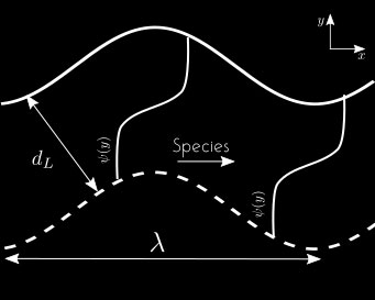
Fig. 6: Mass transport phenomena in the thickness of the flame.
Modification of the local flame speed
In practice, as explained above, these transport phenomena happening in the thickness of the flame tend to modify the local flame speed. Therefore, the assumption made by Darrieus and Landau saying that the flame propagates at the same speed everywhere according to the kinematic relation: $$(\boldsymbol{u}_1-\boldsymbol{w})\cdot\boldsymbol{n}=u_L,$$ — where \(\boldsymbol{u}_1\) is the speed of the unburnt gases, \(\boldsymbol{w}\) the speed of the flame front and \(\boldsymbol{n}\) the normal unit vector to the flame front — does not hold. This was first remarked by Markstein who proposed a new kinematic relation of the form: $$(\boldsymbol{u}_1-\boldsymbol{w})\cdot\boldsymbol{n}=u_L-\mathcal{L}\kappa,$$ where \(\kappa\) is the local curvature of the flame front and \(\mathcal{L}\) is the Markstein length. The latter is a key quantity as it transcribes the influence, of the transport phenomena happening in the flame, on the local flame speed. It allows to take the role of these mass and heat fluxes into account while still considering the flame as a flow discontinuity (interface of infinitesimal thickness).
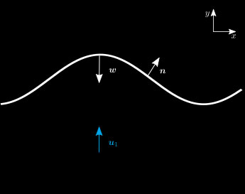
Fig. 7: Local flame speed. The kinematic relation, relating the flame speed \(\boldsymbol{w}\) to the speed of the flow \(\boldsymbol{u}_1\) must take into account the modification of the local flame speed induced by transport phenomena happening in the thickness of the flame.
This kinematic relation first introduced phenomenologically by Markstein can be formally obtained through asymptotic analysis of the internal structure of the flame (see Clavin & Searby (2016) for a review).
For the flames studied here, \(\mathcal{L}>0\), which means the areas of the flame that are behind (negative curvature) propagates faster than the areas that are ahead (positive curvature). Therefore, these transport phenomena tends to stabilize the flame. They introduce a relaxation term of the form \(\sigma=-\Omega u_Lk^2/k_c\) on the growth rate of the perturbation and the dispersion relation becomes of the form: $$\sigma=\Omega u_L(|k|-\frac{k^2}{k_c})$$ where \(k_c\) is the new cutoff wavelength introduced by transport phenomena in the flame. These effects are negligible at large wavelengths compared to the Darrieus-Landau effect introduced earlier (for \(k \ll 1\) the second term vanishes and the Darrieus-Landau growth rate is recovered) and become predominant at small wavelengths. See Joulin & Vidal (1998) for a more detailed introduction to flame front stability).
Non-linear geometrical effect
On vid. 1 and vid. 2 (at the top of this webpage) we can see that the flame front exhibits cellular structures separated by sharp tips whose amplitude remain nearly constant over time. These dynamics result from a competition between the two linear mechanisms described above and non-linear mechanisms that saturate this instability.
The main non-linearity is geometrical and simply comes from the fact that the flame front propagates in the direction perpendicular to itself. In consequence, the concaves part of the front tend to shrink forming sharp structures with strong curvature while the convex parts tend to expand (see Fig. 8).
If the local ordinate of the flame front is described by a function \(\phi(x)\), the flame propagates everywhere in a direction that forms an angle \(\phi_x\) with the vertical direction (where the \(x\) subscript stands for the spatial derivative). In the simplified case where the flame propagates at the speed \(u_L\) everywhere, the variation of the front position in time is then given by \(\phi_t=u_L\cos(\phi_x)\) which in the small slope limit (i.e \(\phi_x\ll 1\)) reduces to: $$\phi_t=u_L(1-\frac{\phi_x^2}{2})+O(\phi_x^4)$$
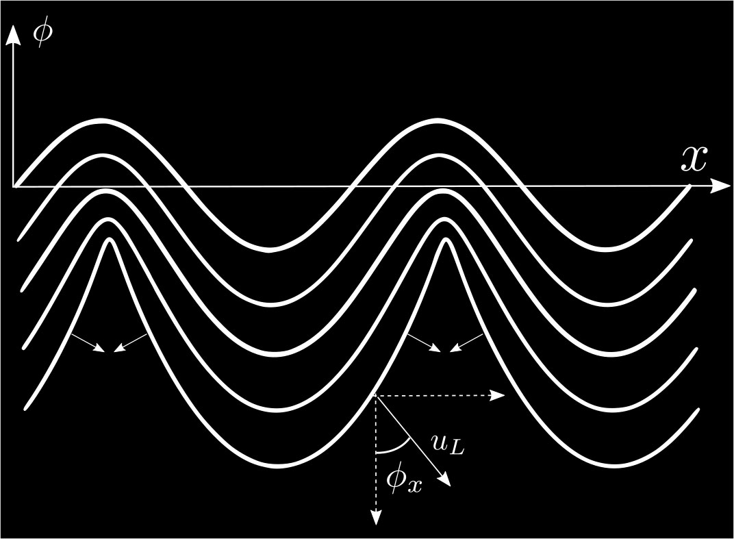
Fig. 8: The quadratic geometrical non-linearity tends to form cellular structure separated by sharp cusps.
As can be seen, the non-linearity associated with this normal propagation is quadratic. This effect, together with the two linear mechanisms described earlier explain the dynamics observed in vid. 1 and vid. 2
Michelson-Sivashinsky equation
A closed equation that includes the three ingredients discussed above can actually be obtained through asymptotic development of the full set of equation in the limit where \(\gamma \ll 1\). As discussed earlier, \(\gamma\) is the parameter that characterizes the density drop experienced by the flow when passing through the flame. The latter is one of the two ingredients that makes the planar flame front configuration unstable. For \(\gamma=0\), the flame front is stable and becomes unstable as soon as \(\gamma>0\). Therefore, \(\gamma=0\) is a bifurcation point of the system and an asymptotic analysis in its very vicinity is likely to provides the essential ingredients involved in the flame dynamics.
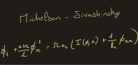
This was first remarked by Sivashinsky who performed the first asymptotic analysis in the small \(\gamma\) limit and obtained the weakly non-linear Michelson-Sivashinky (MS) equation: $$\phi_t+\frac{u_L}{2}\phi_x^2=\Omega u_L\left(I(\phi, x)+\frac{1}{k_c}\phi_{xx}\right)$$ where \(\phi(x,t)\) is a function that describes the altitude of the flame front at location \(x\) and time \(t\) and \(I(\phi,x)\) is a linear operator corresponding to multiplication by \(|k|\) in Fourier space. As can be seen, this equation exhibits the quadratic non-linearity associated with the normal propagation of the front, a linear operator \(I(\phi, x)\) associated with the amplification of perturbations due to the Darrieus-Landau mechanism and a stabilizing term associated with the curvature of the front \(\phi_{xx}\) acting at small wavelength that transcribes the influence of transport mechanisms happening in the thickness of the flame. Linearization of this equation yields the dispersion relation of the form \(\sigma\sim|k|-k^2\) discussed earlier, as it must.
Through proper non-dimensionalisation, this equation can be reduced to: $$\widetilde{\phi}_{\widetilde{t}}+\frac{1}{2}\widetilde{\phi}_\widetilde{x}^2=I(\widetilde{\phi}, \widetilde{x})+\nu \widetilde{\phi}_{\widetilde{x}\widetilde{x}}$$ where the tilded symbols stands for the non dimensional quantities and the single parameter \(\nu\) is called "number of unstable modes" as it corresponds to the number of time the shortest unstable wavelength \(\lambda_c=2\pi/k_c\) can fit in the width of the domain. In the following, we shall drop the tilded symbols with the understanding that all the quantities are non-dimensional.
MS equation vs Burgers equation
This equation is actually nothing but a Burgers equation with an additional instability term: the Darrieus-Landau operator \(I(\phi,x\)). This is easily seen by rewriting the MS equation in term of the slope of the front \(u=\phi_x\) (see Fig. 9) which yields: $$\underbrace{u_t+uu_x=\nu u_{xx}}_{\text{Burgers equation}}+\underbrace{I(u,x)}_{\text{Darrieus-Landau}}$$
This additional term completely modify the dynamics of the front compared to Burgers dynamics. To see that we analyse the role of each term by introducing them sequentially.
Inviscid Burgers equation
We first look at the dynamics described by an inviscid Burgers equation which corresponds to the left hand side of the MS equation only: $$u_t+u u_x=0$$
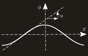
Fig. 9: Rewritting MS equation in term of the slope of the front instead of its vertical position yields a modified Burgers equation.
Due to this non-linear term, the dynamics can lead to formation of singularities (multivalued solution) in a finite time. Here we show an example of the dynamics described by this inviscid Burgers equation starting from a sinusoidal initial configuration. We show both the evolution of the slope \(u\) and the evolution of the vertical position \(\phi\).
Vid. 3: Dynamic evolution of a sinusoidal initial condition according to the inviscid Burgers equation. Here we show both the evolution of the slope \(u\) (Left panel) and the evolution of the vertical position \(\phi\) (Right panel).
On vid. 3, the formation of shocks is readily visible. Once formed, these shocks propagates along the solution with a speed given by conservation laws of the quantity \(u\) through the discontinuity. Large shocks propagate faster than small ones and these dynamics typically lead to fusion of shocks (we shall come back to this later).
Burgers equation
We now look at the dynamics starting from the same initial condition when the viscous term is added to the previous equation : this corresponds to the standard Burgers equation: $$u_t+u u_x=\nu u_{xx}$$ The diffusion term acts specifically in region of sharp gradients and prevents the apparition of shocks. This is demonstrated on vid. 4 where the dynamics at short time is similar to the one described by the inviscid Burgers equation but differs from the latter once sharp gradients regions are formed.
Vid. 4: Dynamic evolution of a sinusoidal initial condition according to Burgers equation. Here we show both the evolution of the slope \(u\) (Left panel) and the evolution of the vertical position \(\phi\) (Right panel).
This is clearly visible on the video where the "shocks" are smoothed out (left panel) and the "cusps" are rounded at the tip (right panel). This is directly associated with presence of a diffusive term. Ultimately, at long time, this diffusive term smoothes out everything and leads to a perfectly flat front. This planar configuration is the only available stationary solution in Burgers dynamics.
MS equation
This is not the case with the Michelson-Sivashinsky equation: $$u_t+u u_x=\nu u_{xx}+I(u,x)$$ where the Darrieus-Landau operator completely modifies the dynamics. As mentioned earlier, the latter amplifies any perturbation with a growth rate inversely proportional to the wavelength of the perturbation. In practice, it competes with the diffusive term and the non-linear term introduced earlier and leads to stationnary solution that are not flat.
Vid. 5: Dynamic evolution of a sinusoidal initial condition according to Michelson-Sivashinsky equation. Here we show both the evolution of the slope \(u\) (Left panel) and the evolution of the vertical position \(\phi\) (Right panel).
As can be seen on the video, the obtained stationnary solution have the typical shape observed on actual flame fronts on vid. 1 and vid. 2 at the top of this webpage.
Pole solutions
The Michelson-Sivashinsky and the Burgers equation both belong to a wider class of PDE that admits analytical solution. These analytical solutions take the form: $$u(x,t)=-2\nu\sum_{n=1}^{2N}\frac{1}{x-z_n(t)},\qquad\phi(x,t)=-2\nu \sum_{n=1}^{2N}\ln\left(x-z_n(t)\right),$$ where \(z_n(t)\) are complex singularities that correspond to the "quasi-shocks" (i.e shocks that are smoothed out by the diffusion term) observed in the numerical solutions of Burgers and MS equations (see vid. 4 and vid. 5).
These singularities typically appear by complex conjugate pairs in order for \(u\) and \(\phi\) to be real. An example of such a solution is plotted on Fig. 10 (we have plotted both the associated \(u\) annd \(\phi\)) for two arbitrary pairs of complex conjugate poles. As can be seen, each pair of pole is associated with a quasi-singularity at the abscissa corresponding to \(x=Re(z)\). The more the imaginary part of the pair of poles is small, the more the quasi-singularity tends to a real singularity (i.e for \(Im(z)\rightarrow 0\), the solution diverges in \(x=Re(z)\)).
Thanks to these analytical solutions, the flame front configuration at a given instant in time is entirely characterized by the number \(N\) of complex conjugate pairs of poles and their position in the complex plane. The dynamic evolution of the front is then described by the trajectories of the poles in the complex plane. The latter are described by a system of ordinary differential equation obtained by injecting the expression of these pole solutions into the Burgers or MS PDE. For MS, these trajectories are given by: $$\dot{z}_{\alpha}=-2\nu\sum_{\alpha \neq \beta}\frac{1}{z_{\alpha}-z_{\beta}}-i\text{sign}(Im(z_{\alpha})),$$
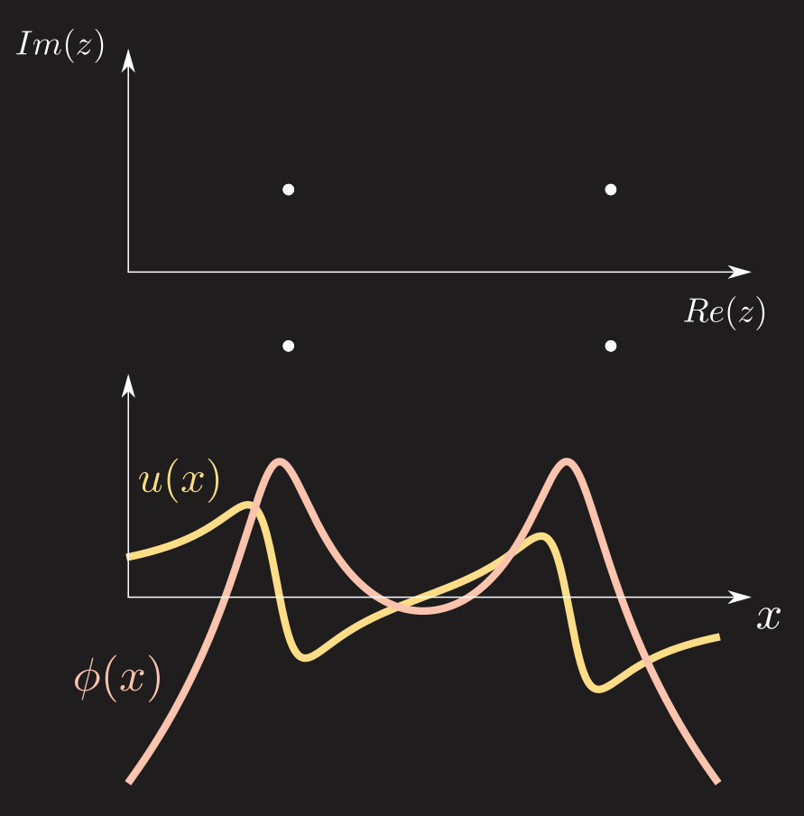
Fig. 10: An example of pole solution with two pairs of complex conjugate poles. The corresponding front \(\phi(x)\) and the corresponding slope \(u(x)\) associated with it, are plotted.
where the index \(\beta\) in the sum goes over all the other existing poles in the complex plane. This dynamical system provides an easy understanding of the flame dynamics observed in vid. 1 and vid. 2.
The second term in this ODE is the easiest to grasp, it simply pulls the poles towards the imaginary axis therefore making deformation of the front more pronounced. It corresponds to the term associated with the Darrieus-Landau instability. Meanwhile, the first term is responsible for a pole to pole attraction along the real axis (horizontal attraction) and a repulsion along the imaginary axis (see Thual et al. (1985)). The resulting dynamics is a complex competition between the attraction towards the real axis that tends to amplify the deformations of the front, the vertical repulsion with complex conjugates that prevents the apparition of singularity on the solution and the horizontal attraction that leads to merging of cusps.
On vid. 6, we show a typical example of this pole dynamics starting from an arbitrary initial condition with periodic boundary conditions. On the upper panel, we have represented the upper half of the complex plane with an initial set of 20 poles spreaded randomly along the real axis. As the poles always appear in complex conjugate pairs, the mirror image of what we are seeing here exists in the lower half of the complex plane (not represented here). On the lower panel of the video, we have represented the front solution \(\phi(x)\) associated with this set of poles. The video then shows the dynamic evolution of this set of poles as described by the set of ODE described earlier (here the ODE system is integrated numerically using a Runge-Kutta 4 integration scheme). As can be seen, in the very first instants, the poles are pulled towards the real axis under the action of the second term in the ODE. This tends to increase the deformations on the front and to form the typical cellular structures separated by sharp tips. The poles are then attracted towards each other along the real axis. This comes from the horizontal pole to pole attraction associated with the first term of the ODE. When they approach each other, these poles tend to pile up on each other due to the repulsive interaction along the imaginary axis. These dynamics induce merging of the associated "cusps" on the front and tend to form larger cusps. Ultimately, all these "cusps" tend to merge in a single giant cusp associated with a single pile of poles.
Vid. 6: Example of pole dynamics (top panel) and the associated front dynamics (bottom panel) starting from an arbitrary initial condition with 20 pairs of complex conjugate poles and periodic boundary conditions. Just note that the real axis line here is thick, letting the reader think that the poles end up on the real axis but they are not. Their imaginary part remains finite at all time due to the vertical repulsion with the complex conjugate.